Implementing NLP XAI

This summarizes part of the project we built for the Hanium ICT competition.

Motivation

While analyzing shopping-mall review data we wanted a differentiator from typical sentiment-analysis models. Specifically, we hoped to highlight the important phrases inside each review. Naver Shopping already highlights key sentences, so we set out to build our own variant.

KeyBERT and similar tools crossed our minds, but the team decided to craft a custom approach. That led us to XAI—if we could calculate which tokens influenced the prediction, we could highlight them automatically.

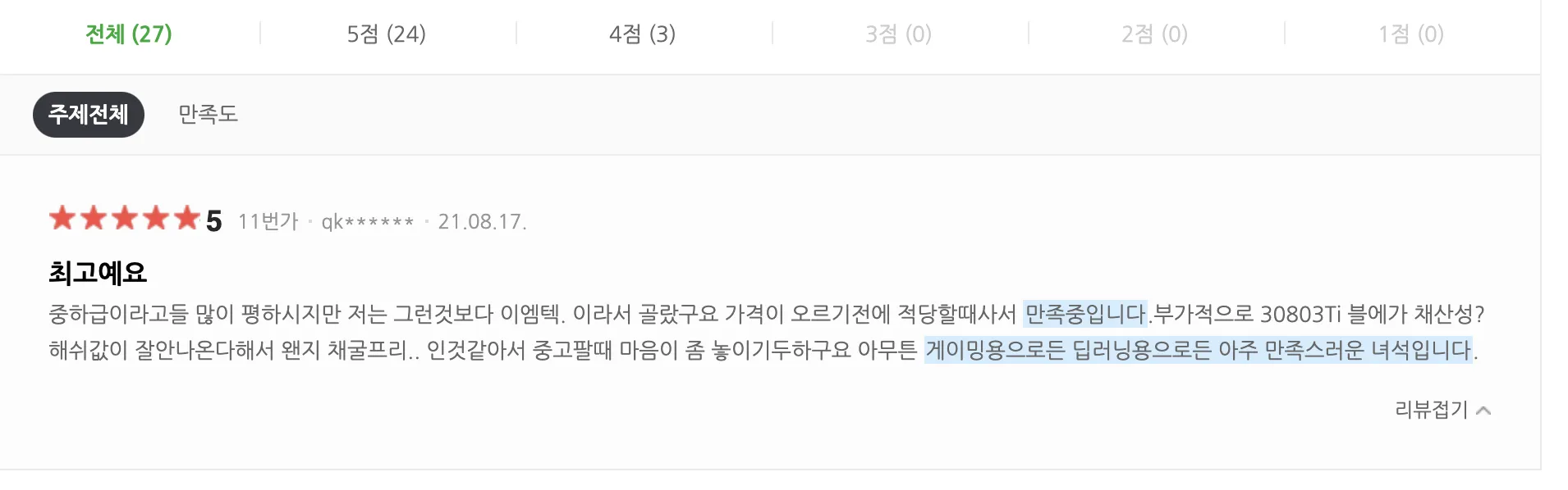
Naver Shopping review highlighting

First Steps with XAI

XAI for NLP proved harder than expected. Computer vision has plenty of open-source explanations; NLP did not. After days of false starts we settled on deriving the influence formula ourselves—compute how each input contributes to the output. Later we discovered the same idea in the Layer-Wise Relevance Propagation (LRP) paper. If only we had found it earlier! The experience taught us to dive into research papers sooner.

Data

Our project revolves around sentiment analysis of shopping reviews. We began with 200K Naver reviews (100K positive with ratings 4–5, 100K negative with ratings 1–2). To boost performance we crawled more data, ending with 540K reviews split evenly between positive and negative.

Morphological Analysis

We chose MeCab. Alternatives like Okt and KKma worked, but MeCab offered better speed, and because shopping reviews often contain slang, Twitter-based training suited us.

Sentence Segmentation

KSS is the go-to Korean sentence splitter, and we used it initially. However, it was too heavy for our service latency. Instead we wrote a lightweight splitter by exploiting sentence endings (“요”, “다”, “죠”) and exceptions like “했음”, “삼”. MeCab’s ETN (nominalizing ending) tag helped. Accuracy isn’t perfect, but speed mattered more for this project.

Stop-Word Removal

Using MeCab we removed particles, sentence endings, prefixes, suffixes, special characters, and unknown tokens.

Word Embedding

Word embedding consumed the most time. We tried Word2Vec + LSTM, but explanation quality disappointed us. So we devised a custom embedding rooted in statistics.

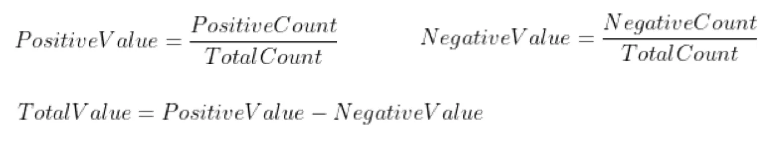
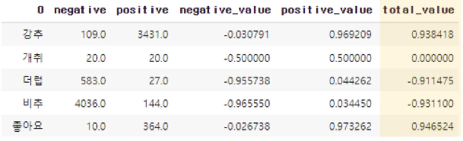
Because we balanced positive and negative samples, we computed the relative frequency of each token within each class. The embedding formula:

(positive frequency / overall frequency) − (negative frequency / overall frequency)

Values range from −1 to 1 (negative tokens near −1, positive tokens near 1).

Model Choice

We eventually used a two-layer DNN. Originally we aimed for Transformer-based XAI, but manually deriving the math was beyond our bandwidth. LSTM also failed our explainability criteria: relevance scores concentrated on trailing tokens. Surprisingly, DNN performed well—LSTM reached 85% accuracy, DNN about 83%. The 2% gap felt acceptable given the explainability gains.

Implementing XAI with LRP

LRP was simpler than expected: propagate relevance from output back to each input using learned weights and biases.

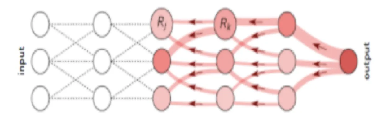
Illustration from the LRP paper

Implementation snippet:

consider_relu = [0 if h < 0 else 1 for h in np.dot(value, weights[0]) + weights[1]]
arr = [
    *map(
        np.sum,
        [
            [
                h * weights[2][index] + weights[3] / (20 * 10)
                for index, h in enumerate(
                    [
                        0
                        if consider_relu[index] == 0
                        else value[i] * weights[0][i][index] + weights[1][index] / 20
                        for index in range(10)
                    ]
                )
            ]
            for i in range(20)
        ],
    )
]

Full code lives in DNN_func on GitHub.

This produced relevance scores per token (after converting morphemes back into words).

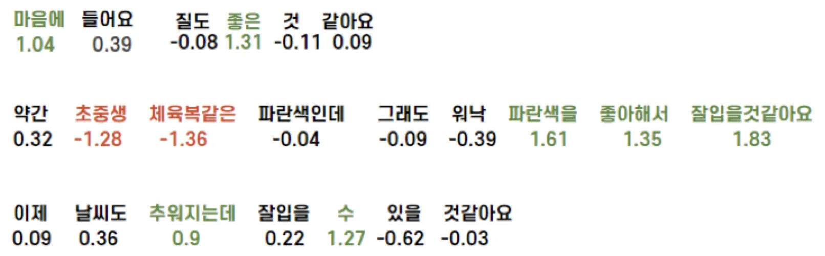
The output looked decent, but we worried users would see disjoint words. We needed post-processing.

Filtering Algorithm

Inspired by CNN filters, we applied sliding-window smoothing. With window size 3 we computed both max and min values; then we merged the central value with whichever absolute magnitude was larger.

if max(x[i - 1], x[i], x[i + 1]) > abs(min(x[i - 1], x[i], x[i + 1])):
    x[i] = (max(x[i - 1], x[i], x[i + 1]) + x[i]) / 2
else:
    x[i] = (min(x[i - 1], x[i], x[i + 1]) + x[i]) / 2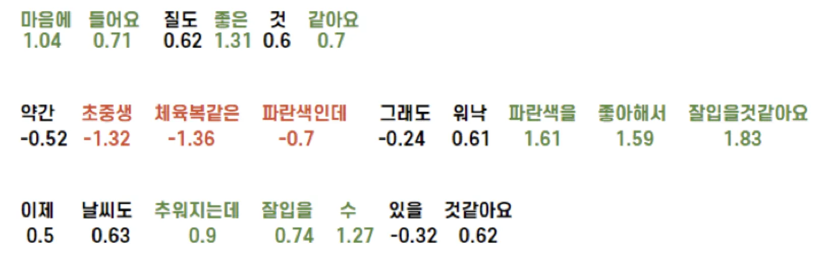

We then tuned thresholds statistically: if the summed relevance exceeded −2.16 we labeled the review positive (green highlight above threshold, red below). Interestingly accuracy rose to 84.3%, surpassing the plain DNN.

Demo

The demo video shows the service in action (note: it’s the mid-term competition submission, so final details differ slightly).